Some Zemax tips and tricks

1. A few useful shortcut keys:

[Ctrl] + z: toggle between turning on and off as a variable.
F3: undo
[Ctrl] + F3: redo
[Ctrl] + a: toggle between multiple configurations.

2. How to show enough digits in the Lens Data Editor:
I prefer to set up at "Compact" mode:
File -> Preferences -> Editors -> Decimals -> Compact.
Or it can be set up to 14 digits.

3. When opening a new window in Zemax, I like to set the window size bigger than Zemax's default:
File -> Preferences -> Graphics -> Window X Size -> 800.
-> Window Y Size -> 600.

4. Add buttons to the tool bar:
File -> Preferences -> Buttons 17-32 (or 33-48)
I added the following which I frequently use:
Qfo (Quick Focus)
Qad (Quick Adjust)
Pop (Physical Optics Propagation)
Gbs (Skew Gaussian Beam)

(Click "Save" button in Preference window to save these custom settings to myZEMAX.CFG).

5. In 3D layout settings, check "Hide Lens Edges" to get the cleaner cross-sectional view (similar to the 2D layout).

6. Never set the # of CPU higher than your PC's actual CPU # (it won't increase Zemax calculation speed).

Gaussian Beam Apodization in Zemax

When the light source in a Zemax model is a Gaussian laser beam, the apodization setting is important.

1. Definition.
From Zemax manual, light amplitude is

A(ρ) = exp(-Gρ2)

Here both A and ρ are the normalized parameters, i.e., they both equal to 0~1 within their full range. G is the apodization factor. If G = 1, the amplitude at the edge of the entrance pupil falls to 1/e of the center value (intensity falls to 1/e²).

2. Determine G value.
From equation:

I(ρ) = exp(-2Gρ2) = 1/exp[2(√ G ρ)2]

It is not difficult to see that entrance pupil (system's clear aperture) radius is √ G times the Gaussian beam's 1/e² radius.

For example, let's plot intensity I vs. ρ at different G values:

From this plot,
(1, blue curve) If G = 1, the Gaussian laser beam is clipped by the system clear aperture right at 13.5% (1/e²) of the peak value. For coherent sources like laser, diffraction will occur significantly.
(2, green curve) If G = 4, the system aperture is twice the size of the beam 1/e² width. This aperture will clip only 0.03% (1/e⁸) of the peak power and should suffice for most laser system.
(3, red curve) If G = 9, the system aperture is three times the size of the beam 1/e² width.

So, the apodization factor determines the Gaussian beam size relative to the system aperture size. If the designer knows both sizes, then setting the G value is easy. For example, for a simple system with a single-mode fiber source and a collimating lens, we know the NA of both. Then the apodization factor should be:

G =

NAlens2 NAfiber2

(1)

Note that the fiber NA in this equation is the 1/e² value. Fiber manufacturers define/measure their NA differently. For example, Corning datasheets give the NA at 1% value, which is 1.517 times larger.

References:
1. http://www.zemax.com/kb/articles/164/1/What-Does-the-Term-Apodization-Mean/Page1.html

Lightroom is limited on color management

Adobe's Lightroom is really great. I now use LR for my 97% of time processing and printing photos. (The remaining 2% time uses Photoshop and 1% uses Silverfast).

However, LR is limited on color management and many times it causes annoying inconvenience:

(1) No soft proofing in LR's print module. For critical printing work, one has to open the file in Photoshop for soft proofing. My 16-bit color images scanned from 8x10 film are 1.5 GB and opening them in both LR and PS can be really slow, if not crashing my computer.

(2) The rendering color profile used in LR's Develop module is ProPhoto RGB but in Library and Print module it is Adobe RGB (1998). Because of this, I have seen some color inconsistency when the image is seen at different LR modules. For example, some deep reds cannot be shown in Adobe RGB color space.

I guess Adobe does not want LR to reduce too much users from PS so they purposely make the LR imperfect... sigh.

A Zemax Case

I had a design using a prism pair to circularize laser diode's elliptical beam. The theoretical plot is below:



The prism positions are designed for 488nm, wavelengths deviating from 488nm will have some beam walk-off (both displacement and steering). Now I want to know how much I need to twist the prism pair for correcting the beam walk-off. The pivot point of twisting is a pin at somewhere not far from the prisms. (Twist the two prisms together since this is a sub-assembly).

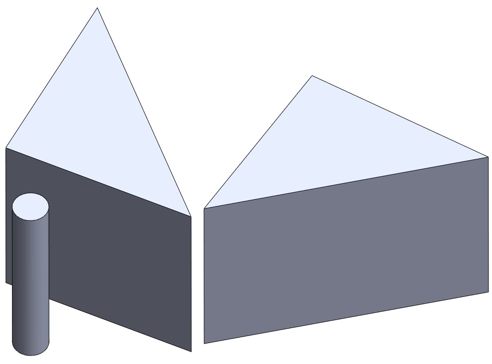
To simulate it in Zemax, I first draw the prisms in SolidWorks with the pivot pin:



Note that in SolidWorks I make the origin point at the pin location. Then I Save As the model in IGS format, to folder C:\Program Files\ZEMAX\Objects\CAD Files. After Zemax imports this file, the reference point is at the pin, which is what I wanted. I found that saving as STL file won't keep the reference point at the same location as in SolidWorks.

Below is the Zemax screen capture. It is a non-sequential model. I can rotate two prisms together around the pin location in Zemax. Beam compression, displacement and steering can all be checked. (Click on images to see in full size.)

Basic of basics of polarization and reflection.

Once upon a time these were taught in college; but I need to refresh them in my mind every once in a while.

p and s polarization: (forget about their Greek/German/? equivalent) Here p means "plunge", s means "stick". Because p light is easier to penetrate (plunge into water) whereas s light is easier to be reflected (a stick bounced from water).

At Brewster angle, the reflected beam is purely s-polarized, meaning the p-polarized light has zero reflectance. Wikipedia [1] has an excellent image to show this effect:



Reflectance vs incident angle is below (for 532nm and fused silica):

At Brewster angle (~56^o), reflectance of s-polarization is about 14%.

References and notes
[1] http://en.wikipedia.org/wiki/Polarizer

Using Zemax as a calculator to calculate for Gaussian beam

Using Zemax to calculate for Gaussian beam propagation is handy and precise.

First set up your optical system in sequential mode. For example, a lens comprised of two surfaces. Here I have a diode window and a collimating lens:



Go to Analysis -> Physical Optics -> Paraxial Gaussian Beam, or simply Ctrl-B. A "Paraxial Gaussian Beam Data" window appears. Click Settings, or right click mouse, the setting menu appears.

Zemax asks for 4 initial values to define the input Gaussian beam:
(1)Wavelength: defined in "Wav" tab.
(2)Waist size: this is 1/e² radius value. Note that this is for the embedded ideal Gaussian beam.^{Note 1}
(3)M² factor: the true Gaussian beam has Mx beam radius and Mx divergence compared to the embedded ideal Gaussian beam.
(4)Waist location.



After hitting OK, the "Paraxial Gaussian Beam Data" window gives Gaussian beam characteristics on all surfaces^{Note 2}. Both embedded and true Gaussian modes will be given. This is better than calculating by hand or by Matlab code that I used to do.

What would be better: I wish Zemax can creat a drawing showing Gaussian beam's marginal ray.

Notes:
1. To convert your real beam's waist size to its embedded Gaussian beam's waist, divided it by M.
2. This is ideal paraxial result without considering any aberrations on the optics. To see how aberration changes the Gaussian beam size, use "Skew Gaussian Beam" function.

Abbe number and glass code

Abbe number:

V =

nD - 1 nF-nC

(1)

where n_D, n_F and n_C are the refractive indices of the material at the wavelengths of the Fraunhofer D-, F- and C- spectral lines (589.2 nm, 486.1 nm and 656.3 nm respectively). Low dispersion (low chromatic aberration) materials have high values of V [1].

Glass code:
Example of BK7:
517642
n = 1.517
V = 64.2
(both at 587.56 nm) [2]

References:
[1] http://en.wikipedia.org/wiki/Abbe_number
[2] http://en.wikipedia.org/wiki/Glass_code